[Note] Rolling Window Analysis in R

Rolling window analysis is a flexible approach for summarizing relationships in time-ordered or gradient-based data by computing statistics within sliding windows. This note demonstrates a custom implementation in R using the smoking dataset to explore how average weekday smoking amounts vary with age.

Rolling window analysis is a way to summarize data by computing statistics within fixed-length windows that slide across an ordered variable. It is useful for checking whether the relationship between a response and an explanatory variable is stable across the range of the data.

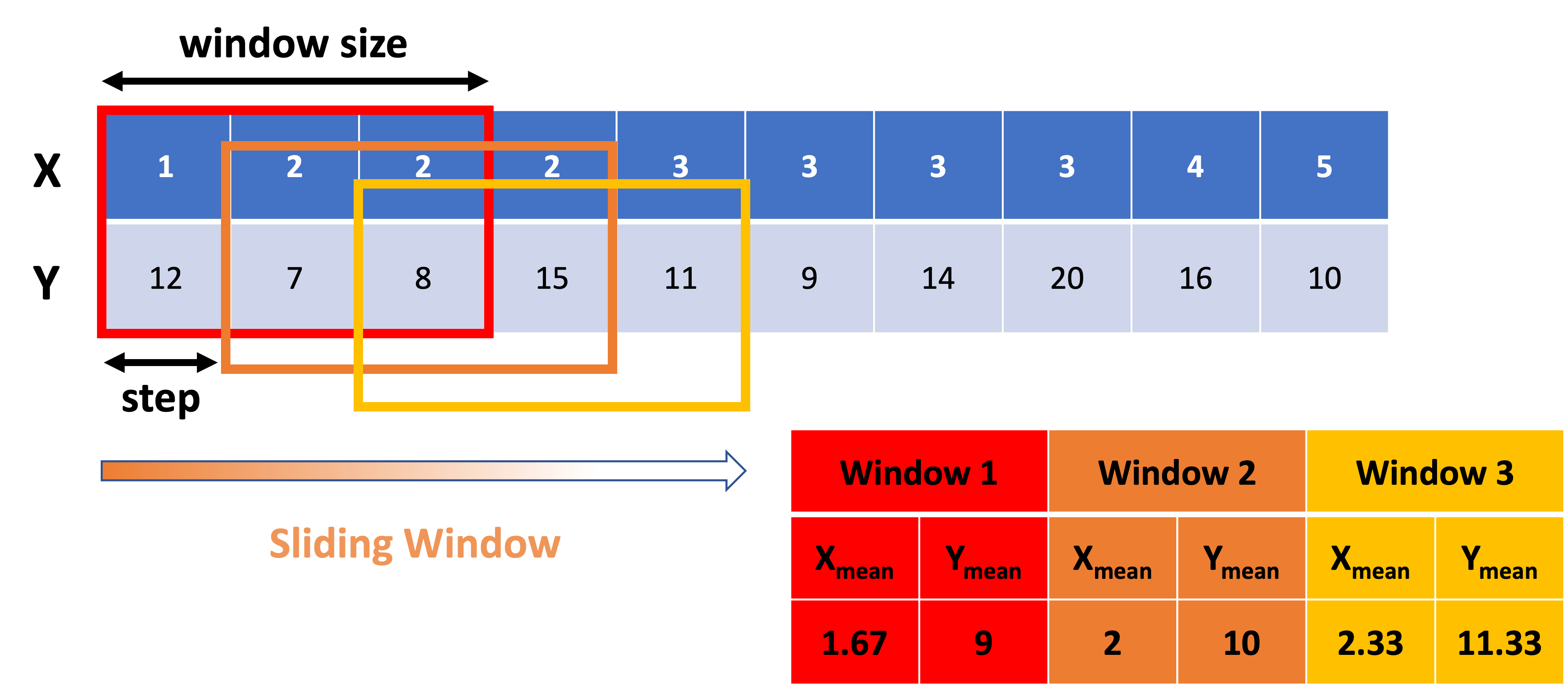
Figure 1. A conceptual figure demonstrating the rolling-window method.

Two key parameters define this method:

• Step size: how far the window moves each iteration
• Window size: how much data each window contains (its span)

Common statistics include mean, standard deviation, and variance.

The zoo package provides rollapply() for rolling calculations, but writing custom code can be more flexible for specific analysis needs.

In this example, we use the smoking dataset from the openintro package to explore the relationship between weekday smoking amount and age.

Dataset documentation:
https://rdrr.io/cran/openintro/man/smoking.html

Data sorting

We first remove missing values and sort the data by age in ascending order.

library(openintro)

data(smoking)

dt = smoking[order(smoking$age), ]
dt = dt[!is.na(dt$amt_weekdays), ]

We visualize the raw relationship:

plot(dt$amt_weekdays ~ dt$age)

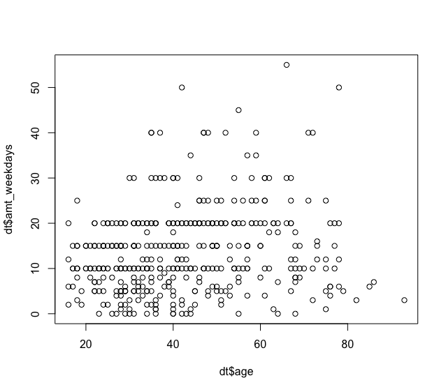
Figure 2. Scatter plot of weekday smoking amount versus age.

Parameter setting

Next, we define the rolling window parameters and prepare a dataframe to store summarized results.

step.age = 0.1     # step size
window.age = 10    # window size

min.age = min(dt$age)
max.age = max(dt$age)

wm.df = data.frame(wm.age = numeric(0),
                   wm.amt_wk = numeric(0))

Writing the loop

The rolling window algorithm computes statistics inside each window, then shifts forward by the step size.

Here we compute the mean age and the mean weekday smoking amount within each window.

i = 0
n_step = (max.age - min.age - window.age) / step.age

for (i in 0:n_step) {

  filter.age = dt$age >= (min.age + i * step.age) &
               dt$age <= (min.age + i * step.age + window.age)

  sub.dt = dt[filter.age, ]

  wm.age = mean(sub.dt$age)
  wm.amt_wk = mean(sub.dt$amt_weekdays)

  wm.dt = list(wm.age, wm.amt_wk)
  wm.df = rbind(wm.df, wm.dt)

  i + 1
}

colnames(wm.df) = c('m.age', 'm.amt_wk')

Plotting

We plot raw data by gender, then overlay the rolling window averages.

library(scales)

filter_f = dt$gender == 'Female'
filter_m = dt$gender == 'Male'

dt$color = as.character(dt$gender)
dt$color[dt$color == 'Female'] = 'pink'
dt$color[dt$color == 'Male'] = 'light blue'

plot(dt$age[filter_m], dt$amt_weekdays[filter_m],
     xlim = c(15, 95), ylim = c(0, 55),
     xaxt = "none", yaxt = "none",
     xlab = "", ylab = "",
     pch = 16,
     col = alpha(unique(dt$color[filter_m]), 0.5),
     tcl = 0.3)

points(dt$age[filter_f], dt$amt_weekdays[filter_f],
       pch = 16,
       col = alpha(unique(dt$color[filter_f]), 0.5))

points(wm.df$m.age, wm.df$m.amt_wk,
       pch = 21, bg = '#FF0033', cex = 2.5)

axis(1, seq(15, 95, 5), las = 1, font = 2)
axis(2, seq(0, 55, 5), las = 2, font = 2)

mtext(side = 1, line = 2, "Age", font = 2)
mtext(side = 2, line = 2, "Number of cigarettes/day", font = 2)
mtext(side = 3, line = 1, "Age dependence of smoking amounts",
      col = "blue", font = 3)

abline(v = c(62.5, 82.5), lwd = 1.2, lty = 2)

legend('topleft',
       legend = c('Female', 'Male', 'Summarized data'),
       pch = 16,
       col = c('pink', 'lightblue', 'red'))

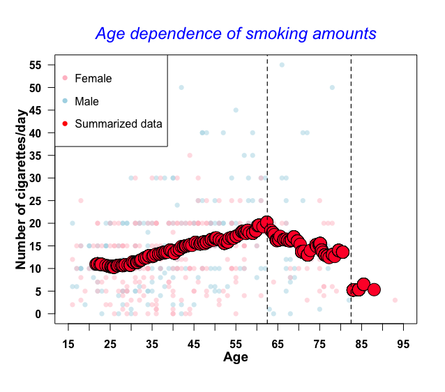
Figure 3. The rolling window averages.

Interpretation

The rolling window summary suggests:

• Ages 20–60: weekday smoking increases with age
• Ages 60–80: weekday smoking decreases with age
• After ~85: weekday smoking drops sharply

This pattern is difficult to see from raw scatter points alone but becomes clear after rolling window smoothing.

Further reading

• rollapply() in the zoo package

END