[Blog] Spatial and Thermal-Stress Dynamics of Native and Introduced Bivalves in the Eastern Scheldt

20 minute read

Published: December 20, 2025

This post documents an end-to-end R workflow that combines long-term benthic surveys (Eastern Scheldt) with mesocosm survival experiments to compare a native cockle and an introduced Manila clam under compound thermal and salinity stress.

Overview

Core components of the pipeline:

Filter large adults to reduce early-life stochasticity and emphasize habitat-integrated survival signals.
Map adult spatial distributions (Google satellite basemap) with fixed abundance classes.
Estimate adult habitat intensity using abundance-weighted KDE.
Quantify temporal persistence (years occupied) per station.
Track abundance-weighted centroid shifts through time.
Model abundance vs. summer thermal extremes using Gamma GLMs.
Derive a compound-stress establishment window from mesocosm survival data.

Project assets (figures + code):

Full workflow script: run_all_bothSpecies.R

Data background

Long-term benthic monitoring in the Eastern Scheldt (Rijkswaterstaat / WMR; curated by Troost et al.) has tracked abundance and distributions of bivalves since 1990. This workflow focuses on 2014–2021, when:

R. philippinarum is fully established across the system,
Temperature records enable explicit quantification of summer heat extremes,
A subset of 111 monitoring stations contains adult individuals of both species, providing a habitat-controlled comparison.

Two focal species:

Native cockle (Cerastoderma edule)
Introduced Manila clam (Ruditapes philippinarum)

Why focus on large adults

Juveniles and larvae are strongly influenced by hydrodynamic transport, storms, and settlement pulses, so their spatial patterns can be noisy and weakly related to habitat quality. By contrast, large adults:

survive ≥ 1–2 winters,
integrate multiple seasons of environmental filtering,
provide stable, interpretable spatial signals.

Size and age class definitions

Cockle (Cerastoderma edule) — age classes

Class	Meaning
1j	1-year-old juvenile
2j	2-year-old
mj	>2-year adult
nb	age undetermined

Large adults = 2j + mj (rare 0j recruits are merged into 1j).

Manila clam (Ruditapes philippinarum) — size classes

Thresholds changed through time:

Years	Small	Large
2014–2017	<1.5 cm	>1.5 cm
2018–2021	<2.0 cm	>2.0 cm

To keep consistency, large adults are identified as “grt” across years (2016 excluded for size-based inference).

Outputs (figures)

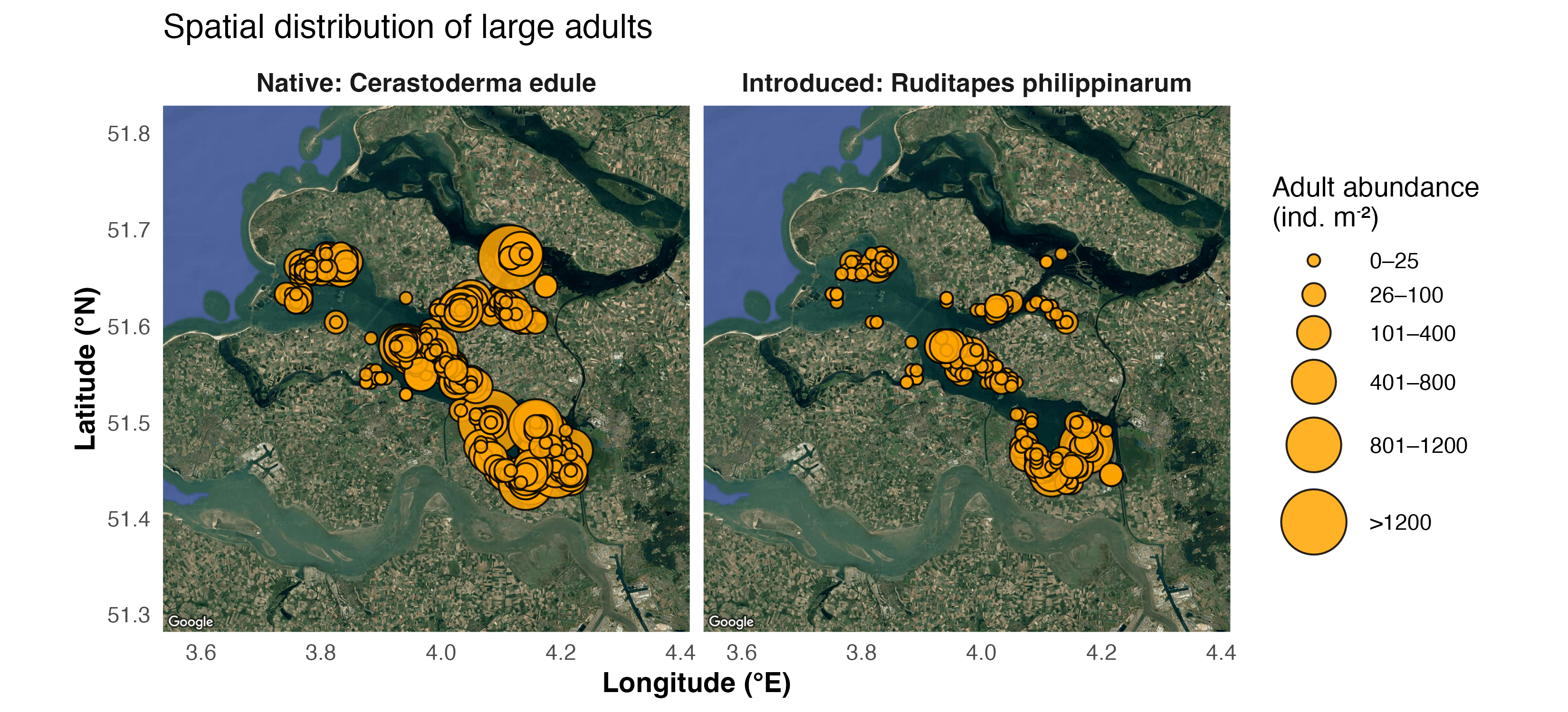Figure 1. Spatial distribution of large adults for native cockles and introduced Manila clams (six abundance classes).

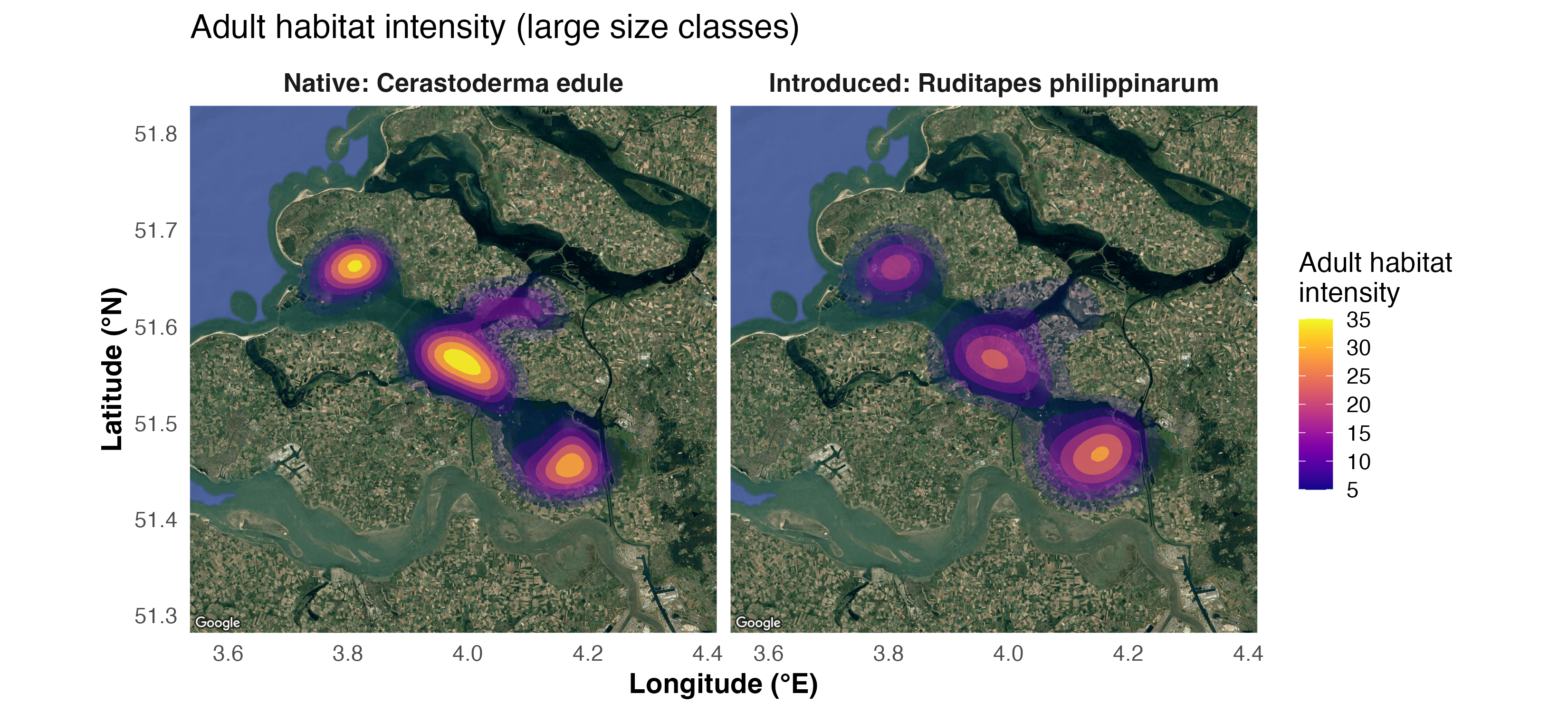Adult habitat intensity (KDE) Figure 2. Adult habitat intensity of large adults (KDE weighted by abundance) for both species.

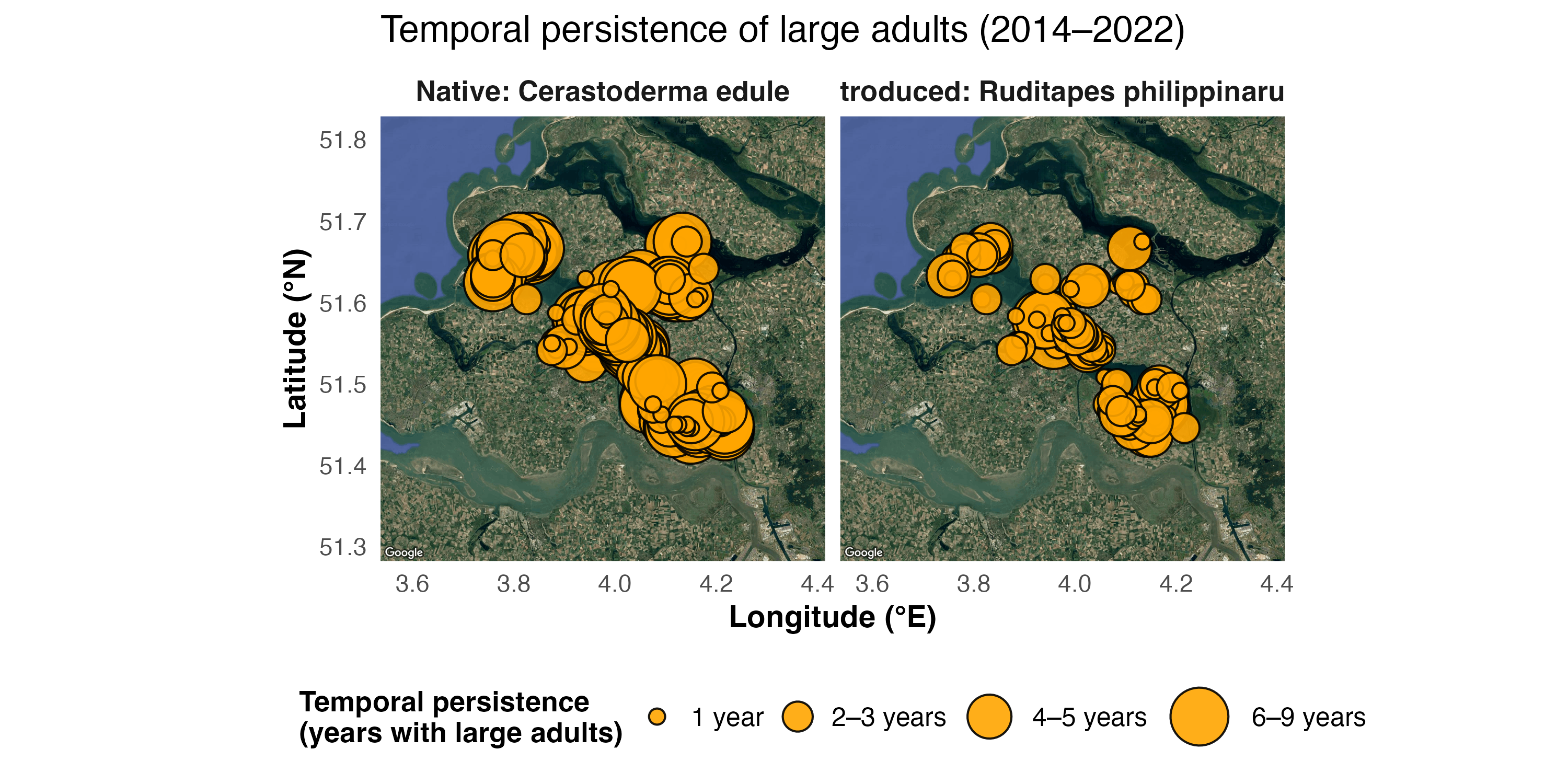Figure 3. Temporal persistence of large adults (years occupied) for both species.

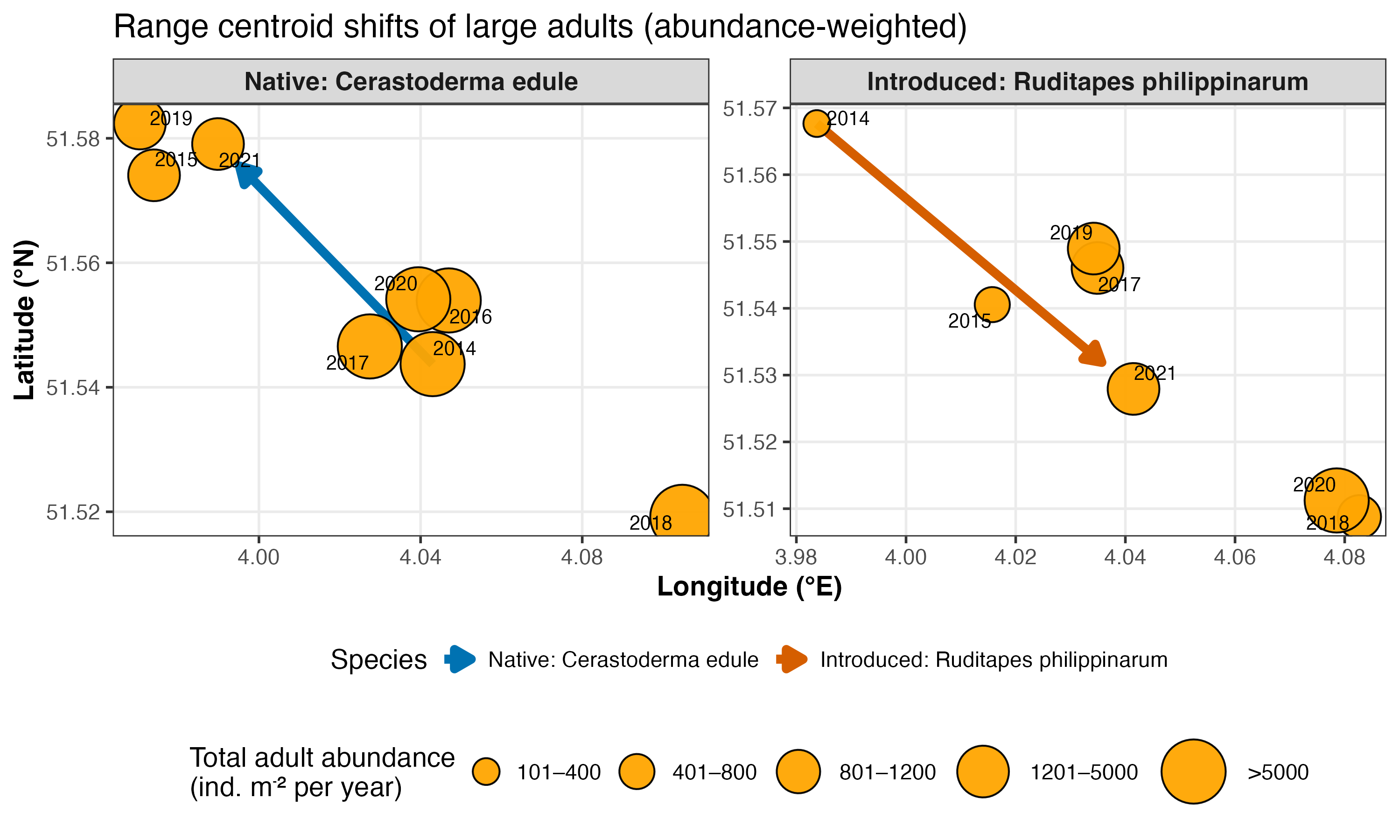Figure 4. Abundance-weighted centroid shifts through time (point size indicates total annual abundance).

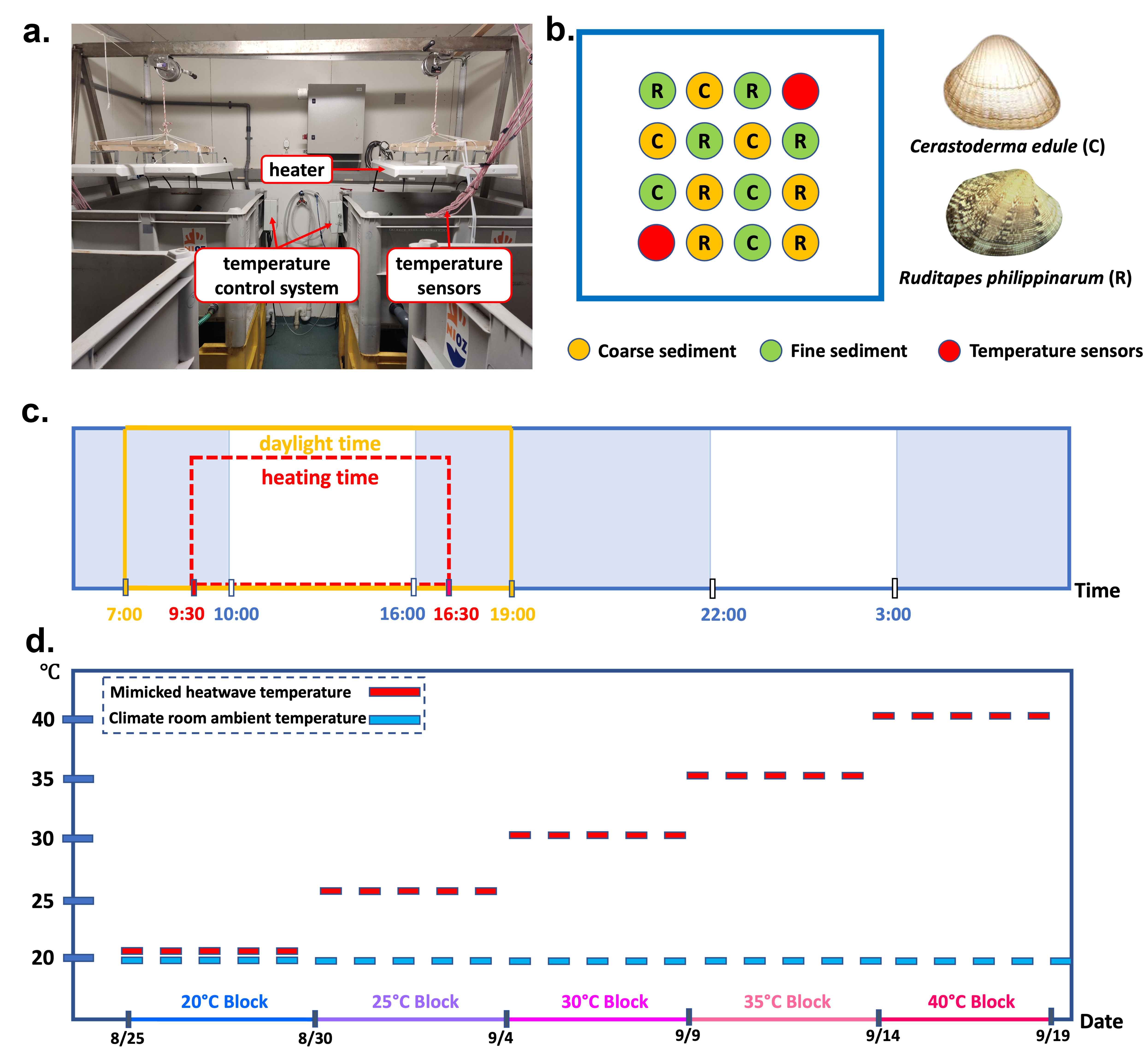Mesocosm setup Figure 5. Mesocosm system used to simulate compound heatwave × salinity stress.

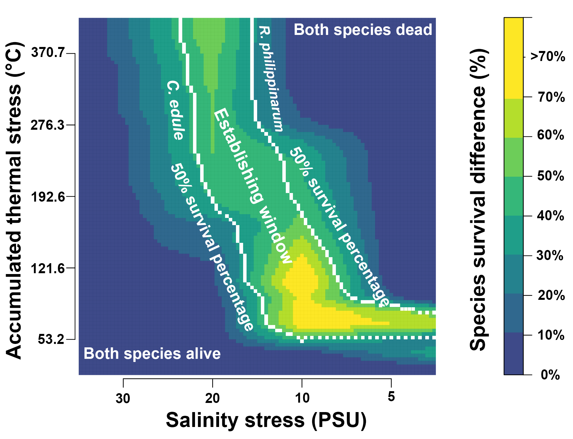Species survival difference window Figure 6. Species survival difference under compound stress, highlighting an establishment window favoring the introduced clam.

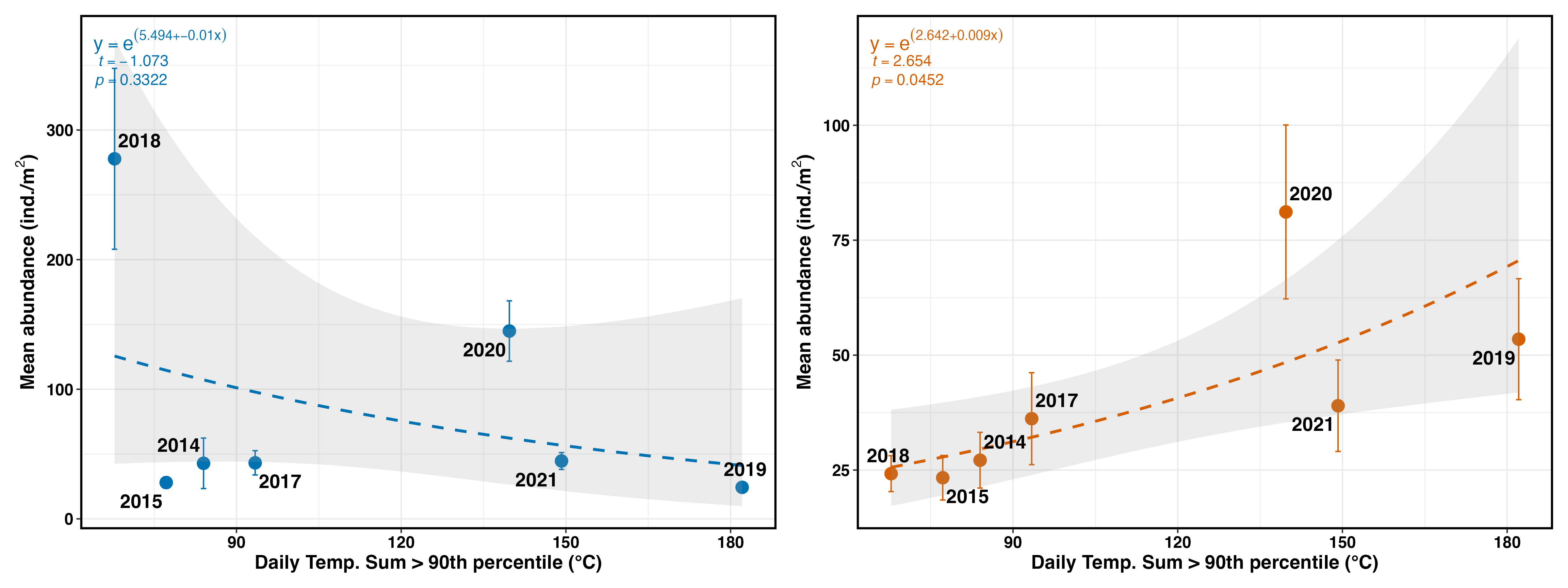Abundance vs temperature extremes Figure 7. Adult abundance vs. summer thermal extremes (daily temperature sum above the 90th percentile), matched to next-year survey abundance.

Tutorial: reproduce the full pipeline (with complete R code)

This section rewrites the full run_all_bothSpecies.R pipeline as a step-by-step tutorial. You can copy/paste sections into an R script or run them interactively.

Files used (expected in your working directory):

Data can be found at this Github repository: bivalve_thermal_thresholds
Field survey data: WMR_WOTdata_OS1421_20221121.xlsx (sheet: data_OS1421)
Temperature data: schiphol70yrs.csv
Mesocosm survival data: sr_2sp.csv

Tip: Run everything at once via:

source("run_all_bothSpecies.R")

0) Setup

Libraries + helper functions

library(readxl)
library(tidyr)
library(dplyr)
library(ggplot2)
library(ggmap)
library(ggrepel)
library(lubridate)
library(patchwork)
library(viridis)
library(zoo)
library(raster)

# simple SE function
std_error <- function(x) sd(x) / sqrt(length(x))

Google Maps basemap (API key)

# Google API key (kept out of script)
google_key <- Sys.getenv("GOOGLE_MAPS_API_KEY")
if (identical(google_key, "") || is.na(google_key)) {
  stop("Please set GOOGLE_MAPS_API_KEY in your environment (e.g. in .Renviron).")
}
register_google(key = google_key)

1) Load and process field data

Load WMR survey data

df.shell <- read_excel("WMR_WOTdata_OS1421_20221121.xlsx", sheet = "data_OS1421")
df.nz    <- df.shell[df.shell$N_m2 != 0, ]

colnames(df.nz)[1] <- "project_id"
colnames(df.nz)[3] <- "station_id"

Subset large adult classes

df.grt <- subset(df.nz, Class %in% c("2j", "mj", "grt"))

Identify year × station entries where both species co-occur

df.grt$year_station <- paste(df.grt$Year,
                             df.grt$station_id,
                             df.grt$Longitude,
                             df.grt$Latitude,
                             sep = "_")

ys_list <- unique(df.grt$year_station)

# this follows your original approach (using an empty template)
df_ysNeo <- df.grt[-(1:1842), ]

for (i in ys_list) {
  df_ys <- df.grt[df.grt$year_station == i, ]
  if (is.element("Cerastoderma edule", df_ys$Species) &&
      is.element("Ruditapes philippinarum", df_ys$Species)) {
    df_ysNeo <- rbind(df_ysNeo, df_ys)
  }
}

Aggregate adult abundance per year × station × species

df_ysNeo$lbs <- paste(df_ysNeo$year_station, df_ysNeo$Species, sep = "_")

lbs_sum <- aggregate(df_ysNeo$N_m2, list(df_ysNeo$lbs), sum)
colnames(lbs_sum) <- c("lbs", "abun")

lbs_sum <- separate(
  lbs_sum,
  col  = lbs,
  into = c("year", "station_id", "longitude", "latitude", "species"),
  sep  = "_"
)

lbs_sum$longitude <- as.numeric(lbs_sum$longitude)
lbs_sum$latitude  <- as.numeric(lbs_sum$latitude)
lbs_sum$year      <- as.numeric(lbs_sum$year)

write.csv(lbs_sum, "lbs_sum.csv", row.names = FALSE)

Prepare a clean adult dataset for mapping

df_adults <- df.grt %>%
  filter(Species %in% c("Cerastoderma edule", "Ruditapes philippinarum")) %>%
  mutate(
    Species = factor(
      Species,
      levels = c("Cerastoderma edule", "Ruditapes philippinarum"),
      labels = c("Native: Cerastoderma edule",
                 "Introduced: Ruditapes philippinarum")
    )
  )

2) Abundance map (both species, 6 classes)

Basemap

bb <- make_bbox(
  lon  = df_adults$Longitude,
  lat  = df_adults$Latitude,
  f    = 0.05
)

base_map <- get_map(
  location = bb,
  source   = "google",
  maptype  = "satellite",
  zoom     = 10
)

Plot

# ---- 6-class abundance scheme (locked-in) ----
df_adults <- df_adults %>%
  mutate(AbundClass = cut(
    N_m2,
    breaks = c(0, 25, 100, 400, 800, 1200, Inf),
    labels = c("0–25", "26–100", "101–400",
               "401–800", "801–1200", ">1200"),
    right  = TRUE
  ))

size_values <- c(2.5, 5, 7.5, 10, 12.5, 15)

p_abund_both <- ggmap(base_map) +
  geom_point(
    data = df_adults,
    aes(x = Longitude, y = Latitude, size = AbundClass),
    shape  = 21,
    fill   = "orange",
    color  = "black",
    alpha  = 0.85,
    stroke = 0.7
  ) +
  scale_size_manual(
    name   = "Adult abundance
(ind. m⁻²)",
    values = size_values
  ) +
  facet_wrap(~ Species) +
  labs(
    title = "Spatial distribution of large adults",
    x = "Longitude (°E)",
    y = "Latitude (°N)"
  ) +
  theme_minimal(base_size = 14) +
  theme(
    strip.text   = element_text(face = "bold", size = 13),
    axis.title.x = element_text(face = "bold"),
    axis.title.y = element_text(face = "bold"),
    panel.grid   = element_blank(),
    legend.position = "right"
  )

p_abund_both

ggsave(
  "abundance_bothSpecies_google_6classes.png",
  p_abund_both,
  width = 11, height = 5, dpi = 300
)

3) Habitat intensity map (KDE intensity, both species)

p_int_both <- ggmap(base_map) +
  stat_density_2d(
    data = df_adults,
    aes(x = Longitude, y = Latitude,
        fill  = after_stat(level),
        alpha = after_stat(level),
        weight = N_m2),
    geom    = "polygon",
    colour  = NA,
    bins    = 8
  ) +
  scale_fill_viridis(
    option = "C",
    name   = "Adult habitat
intensity"
  ) +
  scale_alpha(range = c(0.2, 0.8), guide = "none") +
  facet_wrap(~ Species) +
  labs(
    title = "Adult habitat intensity (large size classes)",
    x = "Longitude (°E)",
    y = "Latitude (°N)"
  ) +
  theme_minimal(base_size = 14) +
  theme(
    strip.text   = element_text(face = "bold", size = 13),
    axis.title.x = element_text(face = "bold"),
    axis.title.y = element_text(face = "bold"),
    panel.grid   = element_blank(),
    legend.position = "right"
  )

p_int_both

ggsave(
  "habitat_intensity_bothSpecies_google.png",
  p_int_both,
  width = 11, height = 5, dpi = 300
)

4) Abundance ~ tempSum regression plots (both species)

# ---- Load temperature data ----
all_70year <- read.csv("schiphol70yrs.csv", header = TRUE)

lbs_sum_corr <- lbs_sum
lbs_sum_corr$label1 <- paste0(lbs_sum_corr$year, "_", lbs_sum_corr$species)

spsYrmean <- aggregate(abun ~ label1, data = lbs_sum_corr, FUN = mean)
spsYrSe   <- aggregate(abun ~ label1, data = lbs_sum_corr, FUN = std_error)
spsYrSd   <- aggregate(abun ~ label1, data = lbs_sum_corr, FUN = sd)
spsYrlnth <- aggregate(abun ~ label1, data = lbs_sum_corr, FUN = length)

spsYrmean <- separate(spsYrmean, label1, into = c("year", "sps"), "_")
colnames(spsYrmean)[3] <- "abun_mean"

spsYrSe   <- separate(spsYrSe,   label1, into = c("year", "sps"), "_")
colnames(spsYrSe)[3]   <- "abun_se"

spsYrlnth <- separate(spsYrlnth, label1, into = c("year", "sps"), "_")
colnames(spsYrlnth)[3] <- "station_reps"

df_spsAT <- spsYrmean

df_spsAT$abun_se      <- spsYrSe$abun_se

df_spsAT$station_reps <- spsYrlnth$station_reps

# ---- Temperature time series ----
temp_70year <- all_70year[!is.na(all_70year$YYYYMMDD), c(1, 12, 14)]
temp_70year$TN <- temp_70year$TN / 10
temp_70year$TX <- temp_70year$TX / 10

temp_70year$date <- as.Date(as.character(temp_70year$YYYYMMDD),
                            format = "%Y%m%d")

temp_70year <- temp_70year %>%
  mutate(date = ymd(date)) %>%
  mutate(
    year  = year(date),
    month = month(date),
    day   = day(date)
  )

temp1421 <- temp_70year[temp_70year$year >= 2013 & temp_70year$year <= 2022, ]

# 90th percentile threshold
thr_90 <- quantile(temp1421$TX, probs = 0.9, na.rm = TRUE)  # ~23.7 °C

temp30h <- temp1421[temp1421$TX >= thr_90, ]

temp30h$TX30diff <- temp30h$TX - thr_90

sumYear30h <- aggregate(TX30diff ~ year, data = temp30h, sum)

sY30h      <- aggregate(TX30diff ~ year, data = temp30h, length)

sY30h_se   <- aggregate(TX30diff ~ year, data = temp30h, std_error)

sumYear30h$duration   <- sY30h$TX30diff
sumYear30h$stad_error <- sY30h_se$TX30diff
sumYear30h$year_match <- sumYear30h$year + 1

# ---- Match summer temp sums to next-year abundance ----
df_spsAT$TX30diff <- sumYear30h$TX30diff[match(df_spsAT$year, sumYear30h$year_match)]
df_spsAT$duration <- sumYear30h$duration[match(df_spsAT$year, sumYear30h$year_match)]
df_spsAT$TX30diff_se <- sumYear30h$stad_error[match(df_spsAT$year, sumYear30h$year_match)]

df_spsAT$year        <- as.numeric(df_spsAT$year)
df_spsAT$abun_mean   <- as.numeric(df_spsAT$abun_mean)
df_spsAT$abun_se     <- as.numeric(df_spsAT$abun_se)
df_spsAT$TX30diff    <- as.numeric(df_spsAT$TX30diff)
df_spsAT$TX30diff_se <- as.numeric(df_spsAT$TX30diff_se)

df_spsAT_ce <- df_spsAT[df_spsAT$sps == "Cerastoderma edule", ]
df_spsAT_rp <- df_spsAT[df_spsAT$sps == "Ruditapes philippinarum", ]

# ---- Gamma GLMs ----
glm_model_ce <- glm(abun_mean ~ TX30diff,
                    data   = df_spsAT_ce,
                    family = Gamma(link = "log"))

glm_model_rp <- glm(abun_mean ~ TX30diff,
                    data   = df_spsAT_rp,
                    family = Gamma(link = "log"))

coef_intercept_ce <- round(coef(glm_model_ce)[1], 3)
coef_slope_ce     <- round(coef(glm_model_ce)[2], 3)

coef_intercept_rp <- round(coef(glm_model_rp)[1], 3)
coef_slope_rp     <- round(coef(glm_model_rp)[2], 3)

glm_summary_ce <- summary(glm_model_ce)
t_value_ce     <- round(glm_summary_ce$coefficients[2, "t value"], 3)
p_value_ce     <- round(glm_summary_ce$coefficients[2, "Pr(>|t|)"], 4)

glm_summary_rp <- summary(glm_model_rp)
t_value_rp     <- round(glm_summary_rp$coefficients[2, "t value"], 3)
p_value_rp     <- round(glm_summary_rp$coefficients[2, "Pr(>|t|)"], 4)

# ---- Regression plots ----
plot1 <- ggplot(df_spsAT_ce, aes(x = TX30diff, y = abun_mean)) +
  geom_point(size = 4, color = "#0072B2") +
  geom_errorbar(aes(ymin = abun_mean - abun_se,
                    ymax = abun_mean + abun_se),
                width = 1.0, color = "#0072B2") +
  geom_errorbarh(aes(xmin = TX30diff - TX30diff_se,
                     xmax = TX30diff + TX30diff_se),
                 height = 1.0, color = "#0072B2") +
  geom_smooth(aes(group = 1),
              method = "glm",
              method.args = list(family = Gamma(link = "log")),
              se = TRUE, linetype = "dashed",
              color = "#0072B2", alpha = 0.2) +
  geom_text_repel(aes(label = year),
                  size = 5, fontface = "bold",
                  box.padding = 0.5, point.padding = 0.6,
                  max.overlaps = Inf) +
  labs(
    x = "Daily Temp. Sum > 90th percentile (°C)",
    y = expression(bold("Mean abundance (ind./m"^2*")"))
  ) +
  annotate("text", x = -Inf, y = Inf,
           label = paste0("y == e^(", coef_intercept_ce, " + ", coef_slope_ce, " * x)"),
           hjust = -0.1, vjust = 1.5, size = 5,
           color = "#0072B2", parse = TRUE) +
  annotate("text", x = -Inf, y = Inf,
           label = paste0("italic(t) == ", t_value_ce),
           hjust = -0.25, vjust = 4.5, size = 4,
           color = "#0072B2", parse = TRUE) +
  annotate("text", x = -Inf, y = Inf,
           label = paste0("italic(p) == ", p_value_ce),
           hjust = -0.20, vjust = 5.1, size = 4,
           color = "#0072B2", parse = TRUE) +
  theme_bw() +
  theme(
    panel.border = element_rect(color = "black", fill = NA, linewidth = 1.5),
    axis.title.x = element_text(size = 14, face = "bold", color = "black"),
    axis.title.y = element_text(size = 14, face = "bold", color = "black"),
    axis.text.x  = element_text(size = 12, face = "bold", color = "black"),
    axis.text.y  = element_text(size = 12, face = "bold", color = "black")
  )

plot2 <- ggplot(df_spsAT_rp, aes(x = TX30diff, y = abun_mean)) +
  geom_point(size = 4, color = "#D55E00") +
  geom_errorbar(aes(ymin = abun_mean - abun_se,
                    ymax = abun_mean + abun_se),
                width = 1.0, color = "#D55E00") +
  geom_errorbarh(aes(xmin = TX30diff - TX30diff_se,
                     xmax = TX30diff + TX30diff_se),
                 height = 1.0, color = "#D55E00") +
  geom_smooth(aes(group = 1),
              method = "glm",
              method.args = list(family = Gamma(link = "log")),
              se = TRUE, linetype = "dashed",
              color = "#D55E00", alpha = 0.2) +
  geom_text_repel(aes(label = year),
                  size = 5, fontface = "bold",
                  box.padding = 0.5, point.padding = 0.6,
                  max.overlaps = Inf) +
  labs(
    x = "Daily Temp. Sum > 90th percentile (°C)",
    y = expression(bold("Mean abundance (ind./m"^2*")"))
  ) +
  annotate("text", x = -Inf, y = Inf,
           label = paste0("y == e^(", coef_intercept_rp, " + ", coef_slope_rp, " * x)"),
           hjust = -0.1, vjust = 1.5, size = 5,
           color = "#D55E00", parse = TRUE) +
  annotate("text", x = -Inf, y = Inf,
           label = paste0("italic(t) == ", t_value_rp),
           hjust = -0.25, vjust = 4.5, size = 4,
           color = "#D55E00", parse = TRUE) +
  annotate("text", x = -Inf, y = Inf,
           label = paste0("italic(p) == ", p_value_rp),
           hjust = -0.20, vjust = 5.1, size = 4,
           color = "#D55E00", parse = TRUE) +
  theme_bw() +
  theme(
    panel.border = element_rect(color = "black", fill = NA, linewidth = 1.5),
    axis.title.x = element_text(size = 14, face = "bold", color = "black"),
    axis.title.y = element_text(size = 14, face = "bold", color = "black"),
    axis.text.x  = element_text(size = 12, face = "bold", color = "black"),
    axis.text.y  = element_text(size = 12, face = "bold", color = "black")
  )

combined_plot <- plot1 + plot2 + plot_layout(ncol = 2)

combined_plot

ggsave(
  "twoSps_tempSum.png",
  combined_plot,
  width = 16, height = 6, units = "in", dpi = 300
)

5) Centroid shift (clean, both species, global abundance scale)

centroids <- df_adults %>%
  group_by(Species, Year) %>%
  summarise(
    mean_lon   = weighted.mean(Longitude, N_m2, na.rm = TRUE),
    mean_lat   = weighted.mean(Latitude, N_m2, na.rm = TRUE),
    total_abun = sum(N_m2, na.rm = TRUE),
    .groups    = "drop"
  ) %>%
  arrange(Species, Year)

segments <- centroids %>%
  group_by(Species) %>%
  summarise(
    x_start = first(mean_lon),
    y_start = first(mean_lat),
    x_end   = last(mean_lon),
    y_end   = last(mean_lat),
    .groups = "drop"
  ) %>%
  rowwise() %>%
  mutate(
    dx   = x_end - x_start,
    dy   = y_end - y_start,
    frac = 0.9,
    x_end_short = x_start + frac * dx,
    y_end_short = y_start + frac * dy
  ) %>%
  ungroup()

centroids_plot <- centroids %>%
  mutate(
    SizeClass = cut(
      total_abun,
      breaks = c(0, 25, 100, 400, 800, 1200, 5000, Inf),
      labels = c(
        "0–25",
        "26–100",
        "101–400",
        "401–800",
        "801–1200",
        "1201–5000",
        ">5000"
      ),
      right = TRUE
    ),
    SizeClass = factor(
      SizeClass,
      levels = c(
        "0–25",
        "26–100",
        "101–400",
        "401–800",
        "801–1200",
        "1201–5000",
        ">5000"
      )
    )
  )

size_vals_cent <- c(
  "0–25"       = 2.5,
  "26–100"     = 4.0,
  "101–400"    = 6.0,
  "401–800"    = 8.0,
  "801–1200"   = 10.0,
  "1201–5000"  = 12.0,
  ">5000"      = 15.0
)

p_centroid_clean <- ggplot() +
  geom_segment(
    data = segments,
    aes(x = x_start, y = y_start,
        xend = x_end_short, yend = y_end_short,
        color = Species),
    arrow     = arrow(type = "closed", length = unit(0.35, "cm")),
    linewidth = 2.2
  ) +
  geom_point(
    data = centroids_plot,
    aes(x = mean_lon, y = mean_lat, size = SizeClass),
    shape = 21,
    fill  = "orange",
    color = "black",
    alpha = 0.95,
    stroke = 0.7
  ) +
  geom_text_repel(
    data = centroids_plot,
    aes(x = mean_lon, y = mean_lat, label = Year),
    size = 3.5,
    max.overlaps   = Inf,
    box.padding    = 0.25,
    point.padding  = 0.25
  ) +
  scale_size_manual(
    name   = "Total adult abundance
(ind. m⁻² per year)",
    values = size_vals_cent
  ) +
  scale_color_manual(
    name = "Species",
    values = c(
      "Native: Cerastoderma edule"          = "#0072B2",
      "Introduced: Ruditapes philippinarum" = "#D55E00"
    )
  ) +
  facet_wrap(~ Species, scales = "free") +
  labs(
    title = "Range centroid shifts of large adults (abundance-weighted)",
    x     = "Longitude (°E)",
    y     = "Latitude (°N)"
  ) +
  theme_bw(base_size = 14) +
  theme(
    strip.text       = element_text(size = 13, face = "bold"),
    axis.title       = element_text(face = "bold"),
    panel.grid.minor = element_blank(),
    legend.position  = "bottom",
    legend.box       = "vertical"
  )

p_centroid_clean

ggsave(
  "centroid_shift_clean_bothSpecies_globalScale_8classes.png",
  p_centroid_clean,
  width = 10, height = 6, dpi = 300
)

6) Temporal persistence map (both species)

df_persist <- df.grt %>%
  filter(Species %in% c("Cerastoderma edule", "Ruditapes philippinarum")) %>%
  group_by(Species, station_id, Longitude, Latitude) %>%
  summarise(
    years_present = n_distinct(Year),
    .groups = "drop"
  ) %>%
  mutate(
    Species = factor(
      Species,
      levels = c("Cerastoderma edule", "Ruditapes philippinarum"),
      labels = c("Native: Cerastoderma edule",
                 "Introduced: Ruditapes philippinarum")
    )
  )

df_persist <- df_persist %>%
  mutate(
    PersistClass = cut(
      years_present,
      breaks = c(0, 1, 3, 5, 9),
      labels = c("1 year", "2–3 years", "4–5 years", "6–9 years"),
      right = TRUE
    )
  )

persist_sizes <- c(
  "1 year"     = 3,
  "2–3 years"  = 6,
  "4–5 years"  = 9,
  "6–9 years"  = 12
)

p_persist <- ggmap(base_map) +
  geom_point(
    data = df_persist,
    aes(x = Longitude, y = Latitude, size = PersistClass),
    shape = 21,
    fill  = "orange",
    color = "black",
    alpha = 0.9,
    stroke = 0.7
  ) +
  scale_size_manual(
    name   = "Temporal persistence
(years with large adults)",
    values = persist_sizes
  ) +
  facet_wrap(~ Species) +
  labs(
    title = "Temporal persistence of large adults (2014–2022)",
    x = "Longitude (°E)",
    y = "Latitude (°N)"
  ) +
  theme_bw(base_size = 14) +
  theme(
    strip.text       = element_text(size = 13, face = "bold"),
    axis.title       = element_text(face = "bold"),
    panel.grid.minor = element_blank(),
    legend.position  = "bottom",
    legend.box       = "horizontal"
  )

p_persist

ggsave(
  "temporal_persistence_bothSpecies_google.png",
  p_persist,
  width = 11, height = 5, dpi = 300
)

7) Establishment window plot (mesocosm survival differences)

Summary helper

summarySE = function(data=NULL, measurevar,
                     groupvars=NULL, na.rm=FALSE,
                     conf.interval=.95, .drop=TRUE) {
  library(plyr)

  # if na.rm==TRUE, don't count NAs
  length2 = function (x, na.rm=FALSE) {
    if (na.rm) sum(!is.na(x))
    else length(x)
  }

  # for each group's data frame, return N, mean, sd
  datac = ddply(data, groupvars,
                .drop = .drop, .fun = function(xx, col) {
                  c(N = length2(xx[[col]], na.rm = na.rm),
                    mean = mean(xx[[col]], na.rm = na.rm),
                    sd = sd(xx[[col]], na.rm = na.rm))
                },
                measurevar)

  datac <- rename(datac, c("mean" = measurevar))

  datac$se <- datac$sd / sqrt(datac$N)

  ciMult <- qt(conf.interval/2 + .5, datac$N-1)
  datac$ci <- datac$se * ciMult

  return(datac)
}

Load and prepare mesocosm survival data

df = read.csv('sr_2sp.csv')
df$date = as.POSIXct(as.character(df$date), format = '%Y%m%d')
df$mr = 1 - df$sr

df$salinity[df$salinity == '5']  = '5 PSU'
df$salinity[df$salinity == '10'] = '10 PSU'
df$salinity[df$salinity == '20'] = '20 PSU'
df$salinity[df$salinity == '30'] = '30 PSU'
df$salinity = factor(df$salinity, levels = c('5 PSU', '10 PSU', '20 PSU', '30 PSU'))

df$sp_code = df$species
df$species[df$species == 'CE'] = 'C. edule'
df$species[df$species == 'RP'] = 'R. philippinarum'

# subset

dfce = df[df$sp_code == 'CE', ]
dfrp = df[df$sp_code == 'RP', ]

# summary

dfce_summ = summarySE(data = dfce, measurevar = 'sr',
                      groupvars = c('date', 'salinity', 'treatment'),
                      na.rm = TRUE)

dfrp_summ = summarySE(data = dfrp, measurevar = 'sr',
                      groupvars = c('date', 'salinity', 'treatment'),
                      na.rm = TRUE)

df_summ = summarySE(data = df, measurevar = 'sr',
                    groupvars = c('species', 'date', 'salinity', 'treatment'),
                    na.rm = TRUE)

df_summ$sp_ht = paste(df_summ$species, df_summ$treatment, sep = '_')

df_neo = df_summ[, c(1,2,3,4,6)]

df_wide = pivot_wider(df_neo, names_from = "treatment", values_from = "sr")

df_order = df_wide[order(df_wide$species, df_wide$salinity, df_wide$date),]

df_order$C = na.locf(df_order$C)
df_order$H = na.locf(df_order$H)
df_order$Sdiff = df_order$C - df_order$H # optional

# add data categories

plb = c(rep('Phase 1', 5), rep('Phase 2', 5), rep('Phase 3', 5), rep('Phase 4', 5), rep('Phase 5', 5))

df_order$phase = rep(plb, 8)

dsb = paste0('D', 1:25)

df_order$days = rep(dsb, 8)

df_order$days = factor(df_order$days, levels = c(paste0('D', 1:25)))

df_order$salinity = factor(df_order$salinity, levels = c('30 PSU', '20 PSU', '10 PSU', '5 PSU'))

# subset by species

df_odce = df_order[df_order$species == 'C. edule', ]

df_odrp = df_order[df_order$species == 'R. philippinarum', ]

df_odce1 = df_odce[seq(5,100, by = 5),]

df_odrp1 = df_odrp[seq(5,100, by = 5),]

Plot WINDOW (survival-difference surface)

par(mar = c(5,5,4,4),font.axis = 2)
Lraster = raster(array(NA,dim = c(100,100)))

df_odrp$svDiff = df_odrp$H - df_odce$H

df_Diff = df_odrp

df_Diff = df_Diff[,-c(1, 4:6)]

X3 = tapply(df_Diff$svDiff, list(df_Diff$days, df_Diff$salinity), identity)

X3 = X3[nrow(X3):1, ]

sr3 = raster(X3)

sr31 = resample(sr3, Lraster)

sr31[sr31 > 1] = 1
sr31[sr31 < 0] = 0

breakpoints = c(seq(0, 0.7, 0.1), 0.9)

colBW = c(viridis::viridis(10)[3:10], "#FDE725FF")

Phase1 = 53.2
Phase2 = 121.6
Phase3 = 192.6
Phase4 = 276.3
Phase5 = 370.7

png('diff_mRateWINDOW.png',width = 8, height = 6, units='in', res = 300)

plot(sr31, axes = FALSE, box = FALSE, legend = FALSE,
     col = colBW, breaks = breakpoints, zlim = c(0.0,0.9))

plot(rasterToPolygons(sr31), add = TRUE,
     border = adjustcolor("black",alpha.f=0.1) , lwd=1)

axis(side = 1, at = seq(0.125,0.875,length.out = 4), labels = c(30,20,10,5), cex.axis =0.9, pos=-0.01)

axis(side = 2, at = seq(0.1,0.9,length.out = 5), labels = c(Phase1, Phase2, Phase3, Phase4, Phase5), cex.axis =0.9, pos=-0.01)

axis(side = 1, line = 1.5, at = 0.5, labels = 'Salinity stress (PSU)', tick = FALSE, cex.axis = 1.4, pos = -0.08, font = 2)

axis(side = 2, line = 1.5, at = 0.5, labels = 'Accumulated thermal stress (°C)', tick = FALSE, cex.axis = 1.4, pos = -0.1, font = 2)

plot(sr31, axes = FALSE, box = FALSE,
     col = colBW, breaks = breakpoints, zlim = c(0, 0.9),
     legend.width=1.5, legend.shrink=1,
     axis.args=list(at=seq(0.0, 0.9, 0.1),
                    labels=seq(0.0, 0.9, 0.1),
                    cex.axis=0.95, srt = 35),
     legend.args=list(text= expression(bold('Species survival difference')), side=2, font=2, line=1.5, cex=1),
     legend.only=TRUE, horizontal = FALSE)

dev.off()

Citation

Zhou et al. (2025). Compound extreme events reshuffle the stacked odds in the gamble between native and introduced bivalves. Global Ecology and Conservation. DOI

Usage and permissions

All scripts, analyses, and derived figures are intended for academic and non-commercial research use only. Commercial use or public redistribution requires explicit written permission from the authors. Additional restrictions may apply to the original monitoring dataset curated by Rijkswaterstaat / WMR.

Please cite the original publication when using any part of this work.

Share on

Bluesky Facebook LinkedIn Mastodon X (formerly Twitter)

Zhengquan Zhou